Fraction of native contacts over a trajectory

Here, we calculate the native contacts of a trajectory as a fraction of the native contacts in a given reference.

Last executed: Feb 29, 2020 with MDAnalysis 0.20.1

Last updated: January 2020

Minimum version of MDAnalysis: 0.21.0

Packages required:

• MDAnalysis ([MADWB11], [GLB+16])

• MDAnalysisTests

Optional packages for visualisation:

• matplotlib

• pandas

Note

The contacts module contains 3 metrics for calculating the fraction of native contacts for a conformation:

1. hard_cut_q: atoms i and j are in contact if they are at least as close as in the given reference structure

2. soft_cut_q: atoms i and j are in contact based on a soft potential with user-defined parameters ([BHE13])

3. radius_cut_q: atoms i and j are in contact if they are within a given radius ([FKDD07])

import MDAnalysis as mda
from MDAnalysis.tests.datafiles import PSF, DCD
from MDAnalysis.analysis import contacts

import numpy as np
import pandas as pd
import matplotlib.pyplot as plt
%matplotlib inline

Loading files

The test files we will be working with here feature adenylate kinase (AdK), a phosophotransferase enzyme. ([BDPW09]) The trajectory DCD samples a transition from a closed to an open conformation.

u = mda.Universe(PSF, DCD)
ref = mda.Universe(PSF, DCD)

Defining the groups for contact analysis

We define salt bridges as contacts between NH/NZ in ARG/LYS and OE*/OD* in ASP/GLU. You may not want to use this definition for real work.

sel_basic = "(resname ARG LYS) and (name NH* NZ)"
sel_acidic = "(resname ASP GLU) and (name OE* OD*)"
acidic = u.select_atoms(sel_acidic)
basic = u.select_atoms(sel_basic)

Calculating fraction of native contacts, with a distance lower than or equal to the reference structure

contacts.Contacts supports each of the three methods explained above. It must be defined with a selection of two groups that change over time. The fraction of native contacts present in selection are with respect to contacts found in refgroup: two contacting groups in a reference configuration. Native contacts are found in the reference group refgroup based on the radius.

Below, we just use the atomgroups in the universe at the current frame as a reference.

ca1 = contacts.Contacts(u,
                        selection=(sel_acidic, sel_basic),
                        refgroup=(acidic, basic),
                        radius=4.5,
                        method='hard_cut').run()

The results are available as a numpy array at ca1.timeseries. The first column is the frame, and the second is the fraction of contacts present in that frame.

ca1_df = pd.DataFrame(ca1.timeseries,
                      columns=['Frame',
                               'Contacts from first frame'])
ca1_df.head()

	Frame	Contacts from first frame
0	0.0	1.000000
1	1.0	0.492754
2	2.0	0.449275
3	3.0	0.507246
4	4.0	0.463768

Note that the data is presented as fractions of the native contacts present in the reference configuration. In order to find the number of contacts present, multiply the data with the number of contacts in the reference configuration. Initial contact matrices are saved as pairwise arrays in ca1.initial_contacts.

ca1.initial_contacts[0].shape

(70, 44)

You can sum this to work out the number of contacts in your reference, and apply that to the fractions of references in your timeseries data.

n_ref = ca1.initial_contacts[0].sum()
print('There are {} contacts in the reference.'.format(n_ref))

There are 69 contacts in the reference.

n_contacts = ca1.timeseries[:, 1] * n_ref
print(n_contacts[:5])

[69. 34. 31. 35. 32.]

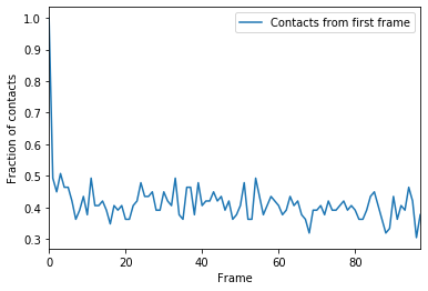
Plotting

ca1_df.plot(x='Frame')
plt.ylabel('Fraction of contacts')

Text(0, 0.5, 'Fraction of contacts')

Calculating fraction of native contacts, with pairs assigned based on a soft potential

refgroup can either be two contacting groups in a reference configuration, or a list of tuples of two contacting groups. Below, we set the reference trajectory to its last frame and select another pair of contacting atomgroups.

ref.trajectory[-1]
acidic_2 = ref.select_atoms(sel_acidic)
basic_2 = ref.select_atoms(sel_basic)

This time we will use the soft_cut_q algorithm to calculate contacts by setting method='soft_cut'. This method uses the soft potential below to determine if atoms are in contact:

\[Q(r, r_0) = \frac{1}{1 + e^{\beta (r - \lambda r_0)}}\]

\(r\) is a distance array and \(r0\) are the distances in the reference group. \(\beta\) controls the softness of the switching function and \(\lambda\) is the tolerance of the reference distance.

Suggested values for \(\lambda\) is 1.8 for all-atom simulations and 1.5 for coarse-grained simulations. The default value of \(\beta\) is 5.0. To change these, pass kwargs to contacts.Contacts.

ca2 = contacts.Contacts(u, selection=(sel_acidic, sel_basic),
                        refgroup=[(acidic, basic), (acidic_2, basic_2)],
                        radius=4.5,
                        method='soft_cut',
                        kwargs={'beta': 5.0,
                                'lambda_constant': 1.5}).run()

Again, the first column of the data array in ca2.timeseries is the frame. The next columns of the array are fractions of native contacts with reference to the refgroups passed, in order.

ca2_df = pd.DataFrame(ca2.timeseries,
                      columns=['Frame',
                               'Contacts from first frame',
                               'Contacts from last frame'])
ca2_df.head()

	Frame	Contacts from first frame	Contacts from last frame
0	0.0	0.999094	0.719242
1	1.0	0.984928	0.767501
2	2.0	0.984544	0.788027
3	3.0	0.970184	0.829219
4	4.0	0.980425	0.833500

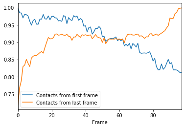
Plotting

Again, we can plot over time.

ca2_df.plot(x='Frame')

<matplotlib.axes._subplots.AxesSubplot at 0x1180755c0>

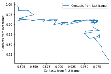
We can also plot the fraction of salt bridges from the first frame, over the fraction from the last frame, as a way to characterise the transition of the protein from closed to open.

ca2_df.plot(x='Contacts from first frame', y='Contacts from last frame')
plt.ylabel('Contacts from last frame')

Text(0, 0.5, 'Contacts from last frame')

References

[1] Oliver Beckstein, Elizabeth J. Denning, Juan R. Perilla, and Thomas B. Woolf. Zipping and Unzipping of Adenylate Kinase: Atomistic Insights into the Ensemble of Open↔Closed Transitions. Journal of Molecular Biology, 394(1):160–176, November 2009. 00107. URL: https://linkinghub.elsevier.com/retrieve/pii/S0022283609011164, doi:10.1016/j.jmb.2009.09.009.

[2] R. B. Best, G. Hummer, and W. A. Eaton. Native contacts determine protein folding mechanisms in atomistic simulations. Proceedings of the National Academy of Sciences, 110(44):17874–17879, October 2013. 00259. URL: http://www.pnas.org/cgi/doi/10.1073/pnas.1311599110, doi:10.1073/pnas.1311599110.

[3] Joel Franklin, Patrice Koehl, Sebastian Doniach, and Marc Delarue. MinActionPath: maximum likelihood trajectory for large-scale structural transitions in a coarse-grained locally harmonic energy landscape. Nucleic Acids Research, 35(suppl_2):W477–W482, July 2007. 00083. URL: https://academic.oup.com/nar/article-lookup/doi/10.1093/nar/gkm342, doi:10.1093/nar/gkm342.

[4] Richard J. Gowers, Max Linke, Jonathan Barnoud, Tyler J. E. Reddy, Manuel N. Melo, Sean L. Seyler, Jan Domański, David L. Dotson, Sébastien Buchoux, Ian M. Kenney, and Oliver Beckstein. MDAnalysis: A Python Package for the Rapid Analysis of Molecular Dynamics Simulations. Proceedings of the 15th Python in Science Conference, pages 98–105, 2016. 00152. URL: https://conference.scipy.org/proceedings/scipy2016/oliver_beckstein.html, doi:10.25080/Majora-629e541a-00e.

[5] Naveen Michaud-Agrawal, Elizabeth J. Denning, Thomas B. Woolf, and Oliver Beckstein. MDAnalysis: A toolkit for the analysis of molecular dynamics simulations. Journal of Computational Chemistry, 32(10):2319–2327, July 2011. 00778. URL: http://doi.wiley.com/10.1002/jcc.21787, doi:10.1002/jcc.21787.