Calculating the root mean square deviation of atomic structures¶

We calculate the RMSD of domains in adenylate kinase as it transitions from an open to closed structure, and look at calculating weighted RMSDs.

Last executed: Feb 06, 2020 with MDAnalysis 0.20.2-dev0

Last updated: January 2020

Minimum version of MDAnalysis: 0.17.0

Packages required:

MDAnalysis ([MADWB11], [GLB+16])
MDAnalysisTests

Optional packages for visualisation:

pandas

Note

MDAnalysis implements RMSD calculation using the fast QCP algorithm ([The05]). Please cite ([The05]) when using the MDAnalysis.analysis.align module in published work.

[1]:

import MDAnalysis as mda
from MDAnalysis.tests.datafiles import PSF, DCD, CRD
from MDAnalysis.analysis import rms

Loading files¶

The test files we will be working with here feature adenylate kinase (AdK), a phosophotransferase enzyme. ([BDPW09]) The trajectory DCD samples a transition from a closed to an open conformation. AdK has three domains:

CORE
LID: an ATP-binding domain
NMP: an AMP-binding domain

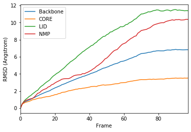
The LID and NMP domains move around the stable CORE as the enzyme transitions between the opened and closed conformations. One way to quantify this movement is by calculating the root mean square deviation (RMSD) of atomic positions.

[2]:

u = mda.Universe(PSF, DCD)  # closed AdK (PDB ID: 1AKE)
ref = mda.Universe(PSF, CRD)  # open AdK (PDB ID: 4AKE)

RMSD between two sets of coordinates¶

The MDAnalysis.analysis.rms.rmsd function returns the root mean square deviation (in Angstrom) between two sets of coordinates. Here, we calculate the RMSD between the backbone atoms of the open and closed conformations of AdK. Only considering the backbone atoms is often more helpful than calculating the RMSD for all the atoms, as movement in amino acid side-chains isn’t indicative of overall conformational change.

[3]:

rms.rmsd(u.select_atoms('backbone').positions,  # coordinates to align
         ref.select_atoms('backbone').positions,  # reference coordinates
         center=True,  # subtract the center of geometry
         superposition=True)  # superimpose coordinates

[3]:

6.8236868672615705

RMSD of a trajectory with multiple selections¶

It is more efficient to use the MDAnalysis.analysis.rms.RMSD class to calculate the RMSD of an entire trajectory to a single reference point, than to use the the MDAnalysis.analysis.rms.rmsd function.

The rms.RMSD class first performs a rotational and translational alignment of the target trajectory to the reference universe at ref_frame, using the atoms in select to determine the transformation. The RMSD of the select selection is calculated. Then, without further alignment, the RMSD of each group in groupselections is calculated.

[4]:

CORE = 'backbone and (resid 1-29 or resid 60-121 or resid 160-214)'
LID = 'backbone and resid 122-159'
NMP = 'backbone and resid 30-59'

[5]:

R = rms.RMSD(u,  # universe to align
             u,  # reference universe or atomgroup
             select='backbone',  # group to superimpose and calculate RMSD
             groupselections=[CORE, LID, NMP],  # groups for RMSD
             ref_frame=0)  # frame index of the reference
R.run()

[5]:

<MDAnalysis.analysis.rms.RMSD at 0x119db9278>

The data is saved in R.rmsd as an array.

[6]:

R.rmsd.shape

[6]:

(98, 6)

R.rmsd has a row for each timestep. The first two columns of each row are the frame index of the time step, and the time (which is guessed in trajectory formats without timesteps). The third column is RMSD of select. The last few columns are the RMSD of the groups in groupselections.

Plotting the data¶

We can easily plot this data using the common data analysis package pandas.

[7]:

import pandas as pd
# the next line is necessary to display plots in Jupyter
%matplotlib inline

We can turn the R.rmsd array into a DataFrame and label each column.

[8]:

df = pd.DataFrame(R.rmsd,
                  columns=['Frame', 'Time (ns)',
                           'Backbone', 'CORE',
                           'LID', 'NMP'])

df

[8]:

	Frame	Time (ns)	Backbone	CORE	LID	NMP
0	0.0	0.000000	7.379926e-07	4.559829e-08	1.137940e-07	7.653031e-08
1	1.0	1.000000	4.636592e-01	4.550182e-01	4.871914e-01	4.745572e-01
2	2.0	2.000000	6.419340e-01	5.754419e-01	7.940987e-01	7.270194e-01
3	3.0	3.000000	7.743983e-01	6.739184e-01	1.010261e+00	8.795031e-01
4	4.0	4.000000	8.588600e-01	7.318859e-01	1.168398e+00	9.612986e-01
...	...	...	...	...	...	...
93	93.0	92.999992	6.817898e+00	3.504430e+00	1.143376e+01	1.029267e+01
94	94.0	93.999992	6.804211e+00	3.480681e+00	1.141134e+01	1.029879e+01
95	95.0	94.999992	6.807987e+00	3.508946e+00	1.137593e+01	1.031958e+01
96	96.0	95.999992	6.821205e+00	3.498082e+00	1.139156e+01	1.037768e+01
97	97.0	96.999991	6.820322e+00	3.507120e+00	1.138473e+01	1.036821e+01

98 rows × 6 columns

[9]:

ax = df.plot(x='Frame', y=['Backbone', 'CORE', 'LID', 'NMP'],
             kind='line')
ax.set_ylabel('RMSD (Angstrom)')

[9]:

Text(0, 0.5, 'RMSD (Angstrom)')

../../../_images/examples_analysis_alignment_and_rms_rmsd_19_1.png

Weighted RMSD of a trajectory¶

Mass¶

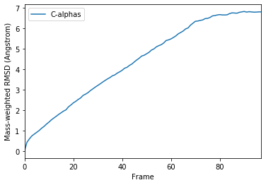
You can also calculate the weighted RMSD of a trajectory using a custom array of weights. (Note: up until version 0.21.0, you cannot calculate the weighted RMSD of groupselections.)

[10]:

R_mass = rms.RMSD(u, u,
                  select='protein and name CA',
                  weights='mass')
R_mass.run()

[10]:

<MDAnalysis.analysis.rms.RMSD at 0x11e61edd8>

[11]:

df_mass = pd.DataFrame(R_mass.rmsd,
                       columns=['Frame',
                                'Time (ns)',
                                'C-alphas'])
ax_mass = df_mass.plot(x='Frame', y='C-alphas')
ax_mass.set_ylabel('Mass-weighted RMSD (Angstrom)')

[11]:

Text(0, 0.5, 'Mass-weighted RMSD (Angstrom)')

../../../_images/examples_analysis_alignment_and_rms_rmsd_24_1.png

Charge¶

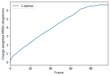
You can also pass in an array of values for the weights. This must have the same length as the number of atoms in select.

[12]:

ag = u.select_atoms('protein and name CA')
ag.charges.shape

[12]:

(214,)

[13]:

R_charge = rms.RMSD(u, u,
                    select='protein and name CA',
                    weights=ag.charges)
R_charge.run()

[13]:

<MDAnalysis.analysis.rms.RMSD at 0x11e5c34e0>

[14]:

df_charge = pd.DataFrame(R_charge.rmsd,
                         columns=['Frame',
                                'Time (ns)',
                                'C-alphas'])
ax_charge = df_charge.plot(x='Frame', y='C-alphas')
ax_charge.set_ylabel('Charge-weighted RMSD (Angstrom)')

[14]:

Text(0, 0.5, 'Charge-weighted RMSD (Angstrom)')

../../../_images/examples_analysis_alignment_and_rms_rmsd_29_1.png

References¶

[1] Oliver Beckstein, Elizabeth J. Denning, Juan R. Perilla, and Thomas B. Woolf. Zipping and Unzipping of Adenylate Kinase: Atomistic Insights into the Ensemble of Open↔Closed Transitions. Journal of Molecular Biology, 394(1):160–176, November 2009. 00107. URL: https://linkinghub.elsevier.com/retrieve/pii/S0022283609011164, doi:10.1016/j.jmb.2009.09.009.

[2] Richard J. Gowers, Max Linke, Jonathan Barnoud, Tyler J. E. Reddy, Manuel N. Melo, Sean L. Seyler, Jan Domański, David L. Dotson, Sébastien Buchoux, Ian M. Kenney, and Oliver Beckstein. MDAnalysis: A Python Package for the Rapid Analysis of Molecular Dynamics Simulations. Proceedings of the 15th Python in Science Conference, pages 98–105, 2016. 00152. URL: https://conference.scipy.org/proceedings/scipy2016/oliver_beckstein.html, doi:10.25080/Majora-629e541a-00e.

[3] Naveen Michaud-Agrawal, Elizabeth J. Denning, Thomas B. Woolf, and Oliver Beckstein. MDAnalysis: A toolkit for the analysis of molecular dynamics simulations. Journal of Computational Chemistry, 32(10):2319–2327, July 2011. 00778. URL: http://doi.wiley.com/10.1002/jcc.21787, doi:10.1002/jcc.21787.

[4] Douglas L. Theobald. Rapid calculation of RMSDs using a quaternion-based characteristic polynomial. Acta Crystallographica Section A Foundations of Crystallography, 61(4):478–480, July 2005. 00127. URL: http://scripts.iucr.org/cgi-bin/paper?S0108767305015266, doi:10.1107/S0108767305015266.